《A Unified Approach to interpreting Model Predictions》论文解读

Introduction #

• 大数据让复杂模型的优势明显
• 提出一种新颖统一的方法用于模型解释
  • 用模型的方法来解释复杂模型（用魔法打败魔法）
  • 提出SHAP值作为各种方法近似统一特征重要度度量
  • 提出新的SHAP值估计方法

Interpretation model properties #

描述解释模型需要有的三个性质，而现在解释方法的缺陷有哪些¹

• 局部准确性：如果x‘是x的简化特征，对应解释模型g(x’) = f(x)，即解释模型在给定的特征情况下能解释为什么模型预测值是这么多。
• 缺失性：当x’=0的时候，贡献度$\phi$为0
• 一致性：模型改变导致特征变的更重要时，贡献度也应该变大

Additive Feature Attribution methods #

一大类方法中解释模型是一系列二元变量的线性函数 称为Additive Feature Attribution methods（AFA）相加特征归因方法 $$g(z’) = \phi_0 + \sum_{i=1}^{M}\phi_i z’_{i}$$ $z’ \in {0, 1}^M$

Classic Shapley Value Estimation #

$$\phi_{i} = \sum_{S \subseteq F\backslash{i}}\frac{|S|!(|F|-|S|-1)!}{|F|!}[f_{S\cup{i}}(x_{S\cup{i}})-f_{S(x_S)}]$$ 基于上面公式精确计算很麻烦，特征的排列有$2^F$种，计算量巨大

SHAP #

SHAP分为模型无关和模型相关两类方法用来近似求解，模型无关的代表是kernelSHAP，而模型相关的代表则有DeepSHAP和TreeSHAP，一个是针对深度学习，一个是针对树模型。

Kernel SHAP #

LIME #

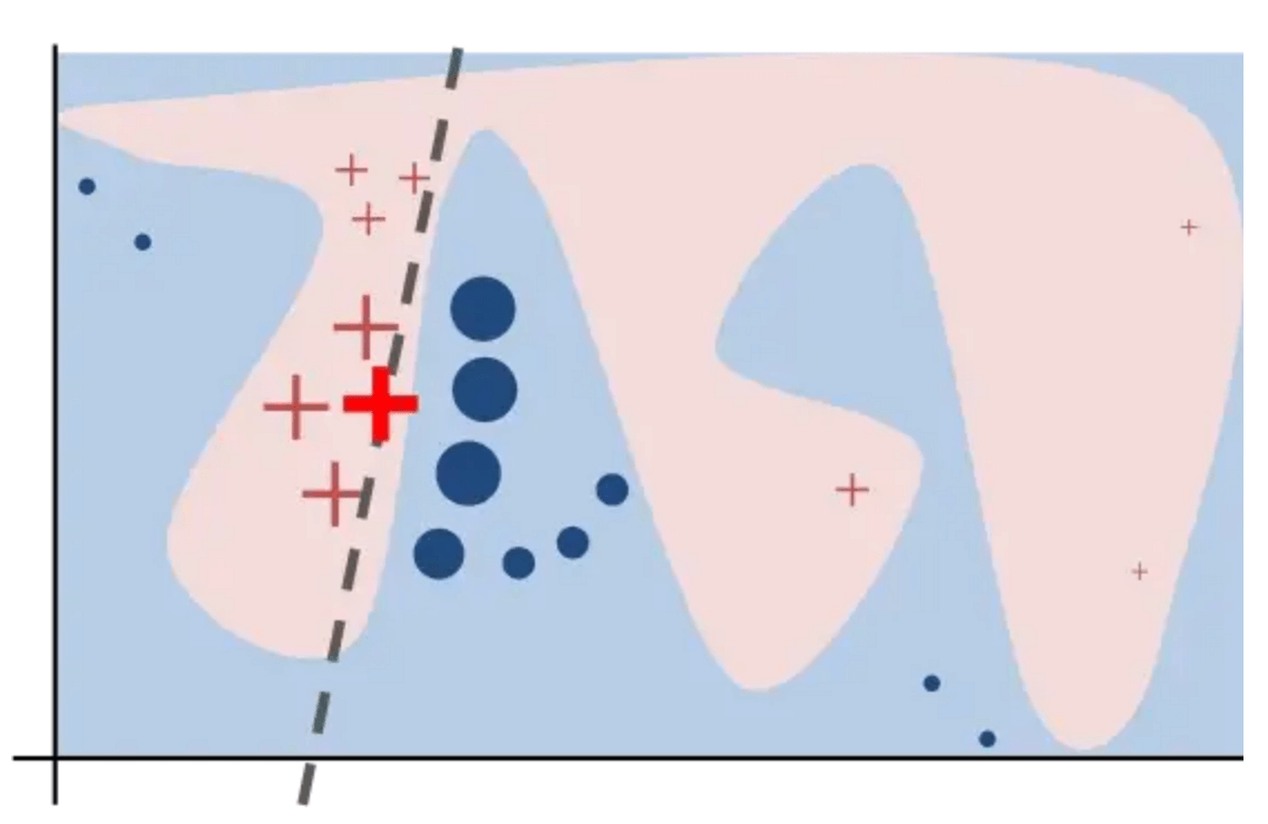
LIME²（Local interpretable model-agnostic explanations)（why should I trust you: Explaining the predictions of any classifier）通过生成的包含需要解释点周围的扰动数据和基于黑箱模型预测结果的数据集，训练一个可以解释的模型，比如逻辑回归、决策树，这个可解释模型需要在解释点周围达到较好的效果。 $$\xi = \mathop{\arg\min}\limits_{g\in G}L(f,g,\pi_x) + \Omega(g)$$

• f为需解释模型
• g为可能的解释模型
• $\pi_x$为定义实例周围多大范围

算法过程：

• 选择需要解释感兴趣的实例
• 对其进行扰动，并得到黑箱模型对应结果产生新数据集
• 根据与实例的接近程度，对新数据集进行赋予权重
• 基于新数据集和上述损失函数求解可解释模型
• 解释预测值

  

  Figure 3: Toy example to present intuition for LIME

KernelSHAP（Linear LIME + Shapley value） #

LIME（Local interpretable model-agnostic explanations）方法的拓展，通过修改LIME需要求解loss等式参数，其主要思路是利用核变换，让$\phi$符合shapley value³ 算法过程⁴：

• 根据$z_k^{’} \in {0, 1}^M$选择k个样本
• 将$z_k^{’} \in {0, 1}^M$转化为原始特征值并计算黑箱模型预测值
• 基于SHAP kernel计算$z_k^{’}$ 样本权重，$z_k$里面1的个数不一样权重就不一样
• 拟合线性模型
• 从线性模型中返回Shapley values SHAP核为(推导过程见2补充材料)： $$\pi_{x’}(z’)= \frac{(M-1)}{(M choose |z’|)|z’|(M-|z’|)}$$ $$L(f,g, \pi_{x’})=\sum_{z’\in Z}[f(h_x^{-1}(z’))-g(z’)]^2\pi_{x’}(z’)$$ x’为简化输入，$x=h_x(x’)$, $z’ \subseteq x’$ 其中第二步：The function h maps 1’s to the corresponding value from the instance x that we want to explain. For tabular data, it maps 0’s to the values of another instance that we sample from the data. This means that we equate “feature value is absent” with “feature value is replaced by random feature value from data”.

Deep SHAP #

DeepLIFT（Learning Important FeaTures） #

DeepLIFT⁵方法使用神经元的激活与其“参考”进行比较，其中参考是神经元在网络获得“参考输入”时具有的激活状态（参考输入根据具体任务的内容定义）。该方法赋予每个特征重要度分数之和等于预测值与基于参考输入的预测值之间的差异⁶。 能解决基于梯度方法的不足，例如参考的差异不是0的情况下梯度仍然可能是0。 $$\sum_{i=1}^n C_{\Delta x_i \Delta t} = \Delta t \tag1$$ $\Delta t = t - t^0$, 神经元输出与参考输出的差异，$\Delta x$输入相对参考输入的变化， C即特征的贡献

$$m_{\Delta x\Delta t} = \frac{C_{\Delta x\Delta t}}{\Delta x} \tag2$$ 定义乘子multiplier，满足链式法则 算法步骤⁷：

• 定义参考值
  • choosing a good reference would rely on domain-specific knowledge, and in some cases it may be best to compute DeepLIFT scores against multiple different references
  • 比如图像用全0或者模糊版本，基因数据用本底期望频率
• 区分正负贡献（2019）
• 贡献度规则
  • 线性层直接是系数$w* \Delta x_i$
  • 非线性变化是$m_{\Delta x\Delta y} = \frac{C_{\Delta x\Delta y}}{\Delta x} =\frac{\Delta y}{\Delta x}$

DeepSHAP(DeepLIFT + Shapley value) #

尽管kernelSHAP是适用于所有模型的包括深度学习模型的一种可解释方法，但是有没有能利用神经网络特性的可解释方法从而提高计算效率。 DeepLIFT计算的分数近似于Shapley value?并不是这个思路

• the Shapely values measure the average marginal effect of including an input over all possible orderings in which inputs can be included. If we define “including” an input as setting it to its actual value instead of its reference value, DeepLIFT can be thought of as a fast approximation of the Shapely values⁸
• Though a variety of methods exist for estimating SHAP values, we implemented a modified version of the DeepLIFT algorithm, which computes SHAP by estimating differences in model activations during backpropagation relative to a standard reference.

  

  

  figure from ref[3]
• 基于Shapley value的定义以及公式可以看出重要的一部分即边际效应，即模型包含该特征减去未包含该部分。在上述一个神经网络模块里面，特征顺序选择都不存在。在认为包含特征即相对于参考输入是真实输入的情况下，把包含特征后乘子直接链式法则做为SHAP值近似公式
• 在上述简单网络组件里面，输入到输出之间可以看作线性近似从而得到公式16
• 把用实际值代替参考值看作是包含某个特征，DeepLIFT方法与DeepSHAP似乎看不到区别?